The most basic form of buckling analysis in FEA is linear buckling. This is directly related to the classic Euler type of calculation. A small displacement perturbed shape is assumed in each element that induces a stress dependent stiffening effect. This adds to the linear static stiffness in the element. Imagine a guitar string tightened – the string total stiffness goes up and results in a higher pitch. If the string is slackened the total stiffness goes down, and the pitch with it. The stress dependent stiffness is now subtracting from the linear static stiffness term. It is this latter effect that causes buckling.
In an assembly of elements in an FEA model there will be a subtle interaction between the original linear stiffness matrix and the stress dependent stiffness matrix. This is analogous to the linear stiffness matrix and the mass matrix in a normal modes analysis. The same solution method is used – an Eigen Value extraction. For a linear buckling analysis this will find what scaling factors applied to the nominal static load will scale the stress stiffening terms to subtract sufficiently from the linear static terms to give unstable solutions.
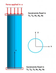
The figure below shows a typical analysis set up. An axial load of a nominal 1KN is applied to the top of a thin walled cylinder. The constraint systems are shown. A linear buckling analysis is carried out. The stress stiffening matrix and the linear static stiffness matrix are calculated in the first linear static step. In the second step the unstable roots are found using the two matrices in an Eigenvalue solution. The user doesn’t have to do anything special here, all buckling solvers are ‘hard-wired’ to do the two steps.
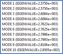
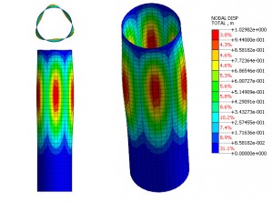
The result of the analysis is a table of eigenvalues as shown in the table above and a set of mode shapes, or eigenvectors. The first mode shape is shown in the figure below.
The critical load that will cause the first buckling mode is calculated from the nominal load (1 KN) multiplied by the eigenvalue (2.575E3 from the table). So the critical load is 2.575E3 KN. We can see the mode shape above. An important question is – can we use the deformation values shown in the figure? The answer is a definite no. Just like a normal modes analysis, all we can get is the shape of the buckled mode. There is no meaning to the values shown in the figure. The length of the cylinder is only 1.5m, so a displacement of 0.8581m as shown would be well beyond any sensible result! We are assuming small displacement perturbations – or shapes. We have no way of allocating displacement values.
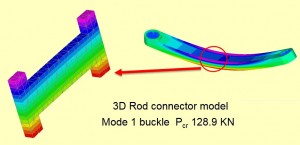
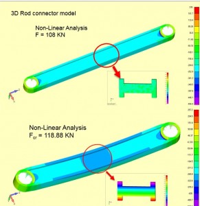
This leads onto a second important question – can we use the stresses calculated from the mode shape, and often shown in a linear buckling analysis? The answer again is a very definite no – for two reasons. The displacements are arbitrary and therefore the strains and stresses are also. The second reason is that the mode shape is only a perturbation normal to the loading axis, so in fact does not couple with the axial load present just before the buckle. This may seem a bit surprising, so I have shown the effect in the figures below. A conrod is analyzed for linear buckling and also for nonlinear buckling. We will go into nonlinear buckling shortly, but basically it allows a continuous load build up and then transition to buckling. The first figure shows a pure bending distribution across the conrod in the linear buckling solution. Clearly there is no contribution from the axial loading. The stress result is meaningless. By contrast the next figure shows a transition of stress in a nonlinear analysis from purely axial just below buckling, to axial plus bending at buckling. The stresses and displacements in the nonlinear case are meaningful.
So coming back to our cylinder, what do we get from the linear buckling analysis? The answer is that we get an estimate of the critical buckling load and the likely mode shape that will result at buckling. We do not know what happens next! Will the cylinder collapse or will it stiffen? What will the final stresses and displacements be? It is rather like a freeze frame photo just at the initiation of buckling – we are left in suspense!
The information we get is very useful in design, but it is more of an indicator than a hard number. We also have to be aware that if we use linear buckling on a structure which is more like the intermediate category, then we are likely to get a non-conservative over estimate of the buckling load. We may also find the mode shape in fact transitions very quickly into something very different.
The boundary condition assumptions for buckling are also critical. However, if the structure can be categorized as ‘slender’ and we can show a good margin over the critical linear buckling load then in many cases that is sufficient for design.
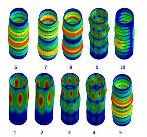
Figure below shows the higher order modes shapes associated with Eigen values 1 to 10. Very often the default in an FEA solver is to just have the first Eigen value and mode shape. In fact the study of the higher modes is useful.
We can see that mode 1 and 2 are identical and represent a repeated mode – any arbitrary axial orientation of the fundamental shape is possible. Modes 3 and 4, 5 and 6, 7 and 8 are also repeated roots. We can also see a distinction between ‘dimpled’ shapes which have a low number of axial lobes and ‘Chinese lantern’ modes which have a high number. The range of eigenvalues is also low – and actually defines critical loads of 2.57E3 to 2.85E3 KN. The implication is that any small variation in boundary condition, component detail or load eccentricity could cause any of the modes to occur. The modes are completely independent in the linear analysis; so mode 1 or 2 or 3 etc. could occur. One way to imagine this is if mode 1 and 2 pair were not possible in practice, by snubbing against adjacent components etc., then mode 3 and 4 pair could occur.
It is important to assess the families of higher mode shapes and Eigen values to see if any practical response implications occur. However often there may be only one dominant first mode, with the next set of modes completely infeasible and at very high critical loads. These can be ignored.
